Bidding Optimization Practice

Q1: Bid Optimization in First-Price Auction for Advertising using Optimization Approach

A company is running an online advertising campaign, bidding on ad placements in a first-price auction. The goal is to determine the optimal bid that maximizes profit while ensuring that total advertising expenditure stays within a specified budget, using the approach discussed in the last lecture.

\text{max} (\text{RPC} - \text{cogs} - \text{CPC})\text{Impressions}\sigma(p(x)f(x, b)) \\ \text{s.t. } \text{CPC} \times \text{Impressions}\sigma(p(x)f(x, b)) \leq \text{Budget} \\ \text{minimum bid} \leq b \leq \text{maximum bid}

Assume there are only two placements: a good place (1) and a bad place (2), and:

Revenue per Click (RPC): Each click on the advertisement generates $5 in revenue.
Cost of Goods Sold (COGS): The cost associated with each click is $1.
Impressions: The ad is ex
pected to be displayed 1,000 times.
Click-Through Rate (CTR): CTR | 𝑋 = 𝑥 ∼ Binomial(𝑝(𝑥))
- p(1) = 0.4 for a good place
- p(2) = 0.6 for a bad place
Function f(x; b) :
- For a good place: $f(x; b) = beta.mean(10, max bid) × b$
- For a bad place: $f(x; b) = beta.mean(3, min bid) × b$
Budget: The total budget for the advertising campaign is $200,000.
Bid Bounds: The bid b must be between $0.01 and$ 4.00.

Write the question in Pyomo.
Find the optimal bid.
Plot the objective function.

1
import pyomo.environ as pyo
2
import numpy as np
3
from scipy.stats import beta
4

5
# parameters
6
rpc = 5
7
cogs = 1
8
impressions = 1000
9
budget = 200000
10
min_bid = 0.01
11
max_bid = 4.0
12

13
# CTR distribution parameters
14
p = {1: 0.4, 2: 0.6}
15
beta_params = {1: (10, max_bid), 2: (3, min_bid)}
16
budget = 200000
17

18
model = pyo.ConcreteModel()
19
model.b = pyo.Var(bounds=(min_bid, max_bid), within=pyo.NonNegativeReals)
20

21

22
def f(x, b):
23
    a, b_param = beta_params[x]
24
    return beta.mean(a, b_param) * b
25

26

27
model.objective = pyo.Objective(expr=(
28
    rpc - cogs - model.b) * impressions * sum(p[x] * f(x, model.b) for x in p), sense=pyo.maximize)
29

30
model.budget_constraint = pyo.Constraint(
31
    expr=model.b * impressions * sum(p[x] * f(x, model.b) for x in p) <= budget)
32

33
solver = pyo.SolverFactory('ipopt')
34
results = solver.solve(model, tee=True)
35

36
optimal_bid = pyo.value(model.b.value)
37

38
print(f"Optimal Bid: ${optimal_bid}")

Output:

1
Optimal Bid: $2.0000000000009908

1
import matplotlib.pyplot as plt
2

3

4
def objective_func(b):
5
    cpc = b
6
    profit = (rpc - cogs - cpc) * impressions * (p[1]*f(1, b) + p[2]*f(2, b))
7
    return profit
8

9

10
bids = np.linspace(min_bid, max_bid, 100)
11
obj_vals = [objective_func(b) for b in bids]
12

13
plt.plot(bids, obj_vals, label="Objective Function")
14
plt.axvline(optimal_bid, color='r', linestyle='--', label="Optimal Bid")
15
plt.xlabel("Bid ($)")
16
plt.ylabel("Objective Function Value")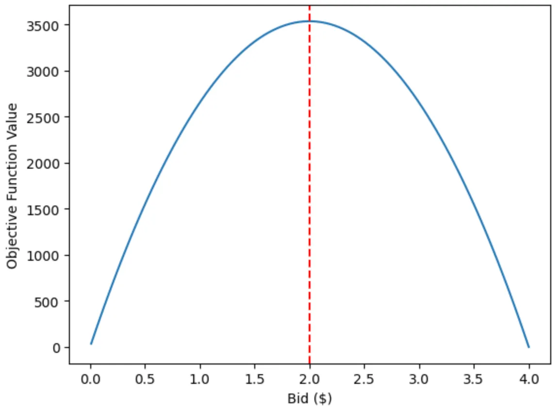

Objective Function Plot

Q2. Bid Optimization in First-Price Auction for Advertising using Multi objective Approach

Assume the same parameters with the following modifications:

$E[CTR] = \frac{bid}{mix\_bid}$ $E[Impressions] = \hat{Impressions} \times \frac{bid}{mix\_bid} \times bid$ $E[Clicks] = E[Impressions] \times E[CTR]$ $P(bid) = (RPC - cogs - CPC) \times E[Clicks]$

We are now considering the problem:

\begin{align*} \max_{b} \quad & \alpha_1 P(b) + \alpha_2 E[CTR] + \alpha_3 E[Impressions] + \alpha_4 E[Clicks] \\ \text{subject to} \quad & E[C(b)] \le Budget \\ & bid_{min} \le b \le bid_{max} \end{align*} \\ \text{where } \alpha_1 + \alpha_2 + \alpha_3 + \alpha_4 = 1

where:

Profit: $\alpha_1 = 0.4$
Expected CTR: $\alpha_2 = 0.2$
Expected Impressions: $\alpha_3 = 0.2$
Expected Clicks: $\alpha_4 = 0.2$

1
import numpy as np
2
import matplotlib.pyplot as plt
3
import pyomo.environ as pyo
4

5
# parameters
6
rpc = 5
7
cogs = 1
8
impressions = 1000
9
budget = 200000
10
min_bid = 0.01
11
max_bid = 4.0
12
p = {1: 0.4, 2: 0.6}
13

14
# weights
15
alpha1, alpha2, alpha3, alpha4 = 0.4, 0.2, 0.2, 0.2
16

17
# helper functions
18

19

20
def f_x_b_good(b):
21
    return beta.mean(10, max_bid) * b
22

23

24
def f_x_b_bad(b):
25
    return beta.mean(3, min_bid) * b
26

27

28
def objective_func(b):
29
    E_ctr_good = b / f_x_b_good(b)
30
    E_ctr_bad = b / f_x_b_bad(b)
31
    E_impression_good = impressions * (b / f_x_b_good(b)) * b
32
    E_impression_bad = impressions * (b / f_x_b_bad(b)) * b
33
    E_clicks_good = E_impression_good * E_ctr_good
34
    E_clicks_bad = E_impression_bad * E_ctr_bad
35

36
    cpc = b
37
    p_bid_good = (rpc - cogs - cpc) * E_impression_good
38
    p_bid_bad = (rpc - cogs - cpc) * E_impression_bad
39

40
    return (alpha1 * (p_bid_good * p[1] + p_bid_bad * p[2]) +
41
            alpha2 * (E_ctr_good * p[1] + E_ctr_bad * p[2]) +
42
            alpha3 * (E_impression_good * p[1] + E_impression_bad * p[2]) +
43
            alpha4 * (E_clicks_good * p[1] + E_clicks_bad * p[2]))
44

45

46
# Compute objective across bids
47
bids = np.linspace(min_bid, max_bid, 200)
48
obj_vals = [objective_func(b) for b in bids]
49

50
# Solve with Pyomo
51
model = pyo.ConcreteModel()
52
model.b = pyo.Var(bounds=(min_bid, max_bid), within=pyo.NonNegativeReals)
53

54
E_ctr_good = model.b / f_x_b_good(model.b)
55
E_ctr_bad = model.b / f_x_b_bad(model.b)
56
E_impression_good = impressions * (model.b / f_x_b_good(model.b)) * model.b
57
E_impression_bad = impressions * (model.b / f_x_b_bad(model.b)) * model.b
58
E_clicks_good = E_impression_good * E_ctr_good
59
E_clicks_bad = E_impression_bad * E_ctr_bad
60
cpc = model.b
61
p_bid_good = (rpc - cogs - cpc) * E_clicks_good
62
p_bid_bad = (rpc - cogs - cpc) * E_clicks_bad
63

64
model.obj = pyo.Objective(expr=alpha1 * (p_bid_good * p[1] + p_bid_bad * p[2]) +
65
                          alpha2 * (E_ctr_good * p[1] + E_ctr_bad * p[2]) +
66
                          alpha3 * (E_impression_good * p[1] + E_impression_bad * p[2]) +
67
                          alpha4 * (E_clicks_good *
68
                                    p[1] + E_clicks_bad * p[2]),
69
                          sense=pyo.maximize)
70

71
model.budget_constraint = pyo.Constraint(
72
    expr=model.b * (E_clicks_good + E_clicks_bad) <= budget)
73

74
solver = pyo.SolverFactory('ipopt')
75
solver.solve(model)
76

77
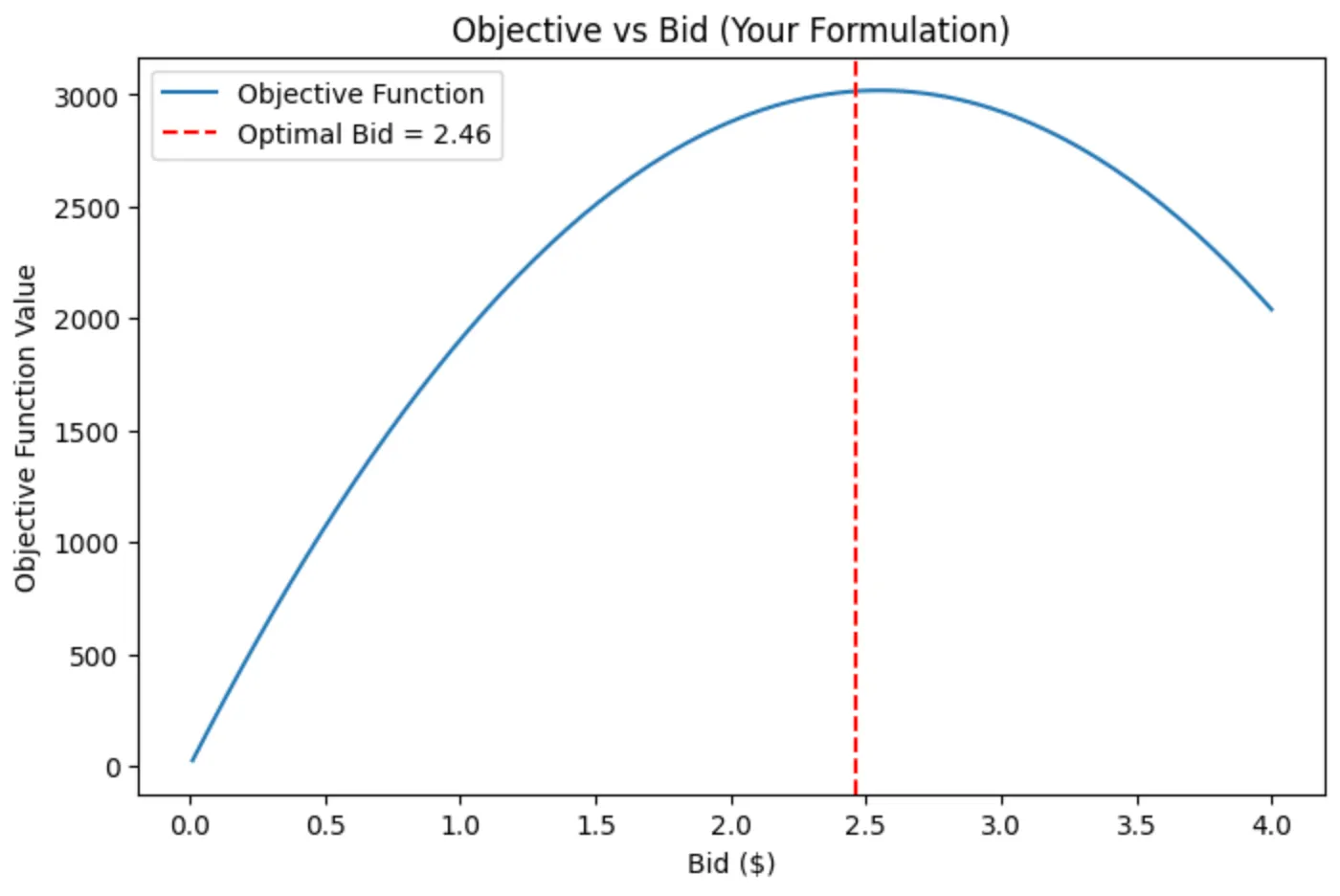
optimal_bid = pyo.value(model.b)
78
print(f"Optimal Bid from Pyomo: ${optimal_bid}")

Output:

1
Optimal Bid from Pyomo: $2.459292942866574

1
# plot
2
plt.figure(figsize=(8,5))
3
plt.plot(bids, obj_vals, label="Objective Function")
4
plt.axvline(optimal_bid, color='r', linestyle='--', label=f"Optimal Bid = {optimal_bid:.2f}")
5
plt.xlabel("Bid ($)")
6
plt.ylabel("Objective Function Value")
7
plt.title("Objective vs Bid (Your Formulation)")
8
plt.legend()
9
plt.show()

Objective Function Plot