Multi-Armed Bandit

Multi-Armed Bandit (MAB) is a sequential decision-making framework used to optimize the allocation of resources among multiple competing options (or “arms”) to maximize cumulative rewards over time. It is particularly useful in scenarios where the true performance of each option is unknown and must be learned through experimentation. It is an adaptive experimentation approach inspired by the problem of a gambler facing multiple slot machines (one-armed bandits) and trying to maximize their total winnings by choosing which machines to play and how often.

In an A/B Testing context, it dynamically allocated traffic to different variations based on real-time performance, balancing exploration (testing less-known options) and exploitation (favoring the best-known option).

Advantages of Multi-Armed Bandit

Dynamic Allocation: Adjusts traffic allocation in real-time, sending more users to better-performing variations, reducing wasted impressions on underperforming options.
Faster Convergence: Reaches conclusions more quickly than traditional A/B testing because it learns and adapts during the test.
Efficient Resource Usage: Maximizes rewards (e.g., clicks or conversions) during the experiment rather than waiting for the test to conclude.
Handles Multiple Variants: Can test more than two versions simultaneously, making it more efficient for multi-variant experiments.
Minimizes Opportunity Cost: Reduces the negative impact of exposing users to underperforming variants by quickly shifting traffic to better options.
Continuous Learning: Operates continuously, making it suitable for long-term optimization and environments with changing user preferences.

Definition

It is a simplified version of Markov Decision Process (MDP), but without state transitions. The goal is to maximize the total reward over a series of trials by choosing from multiple options (arms), each with an unknown reward distribution.

\text{Maximize } \sum_{t=1}^{T} r_t

The optimal reward probability $\theta^*$ of the optimal arm $a^*$ is defined as:

\theta^* = Q(a^*) = \max_{a \in A} E[r | a] = \max_{1 \leq i \leq k} \theta_i

Bandit Strategies

Epsilon-Greedy
Upper Confidence Bound (UCB)
Hoeffding’s Inequality
Bayesian UCB
Thompson Sampling

Epsilon-Greedy Strategy

The Epsilon-Greedy strategy is a simple and effective approach to balance exploration and exploitation in the Multi-Armed Bandit problem. It involves choosing the best-known option most of the time while occasionally exploring other options to gather more information.

Choose each arm once.
Choose arm in round $t$ $t$ : $A_t = \begin{cases} \text{argmax}_{a} \text{Empirical Reward}_i & \text{with probability } 1 - \epsilon_t \\ \text{uniform}(A) & \text{with probability } \epsilon_t \end{cases}$ where $\epsilon_t = \min \{1, \frac{C\times k}{t \times \triangle_{min}^2}\}$ $ϵ_{t} = min {1, \frac{C \times k}{t \times △ _{min}^{2}}}$
- $c$ is a constant that controls the exploration rate
- $k$ is the number of arms
- $t$ is the current time step
- $\triangle_{min}$ is the minimum difference in mean rewards among arms.

Code Example

Epsilon-Greedy Implementation

1
import numpy as np
2
import matplotlib.pyplot as plt
3

4
np.random.seed(42)
5

6
# Epsilon-Greedy Bandit Algorithm
7
class EpsilonGreedyBandit:
8
    def __init__(self, n_arms, c, delta_min):
9
        self.n_arms = n_arms
10
        self.c = c
11
        self.delta_min = delta_min
12
        self.arm_rewards = np.zeros(n_arms) # cumulative rewards for each arm
13
        self.arm_counts = np.zeros(n_arms)  # number of times each arm was pulled
14
        self.total_counts = 0               # total number of pulls
15

16

17
    def calculate_epsilon(self):
18
        total_counts = self.total_counts + 1  # to avoid division by zero
19
        epsilon = min(1, (self.c * self.n_arms) / (self.delta_min ** 2 * total_counts))
20
        return epsilon
21

22
    def select_arm(self):
23
        epsilon = self.calculate_epsilon()
24
        if np.random.rand() < epsilon:
25
            return np.random.randint(self.n_arms)  # Explore
26
        else:
27
            return np.argmax(self.arm_rewards / (self.arm_counts + 1e-5))  # Exploit
28

29
    def update(self, arm, reward):
30
        self.arm_rewards[arm] += reward
31
        self.arm_counts[arm] += 1
32
        self.total_counts += 1
33

34
# Simulation three ads with different reward distributions
35
true_mean_rewards = [0.3, 0.5, 0.7]
36
reward_distributions = [lambda: np.random.binomial(1, p) for p in true_mean_rewards]
37

38
# Parameters
39
n_arms = len(true_mean_rewards)
40
c = 1
41
delta_min = min(true_mean_rewards)
42

43
# Initialize bandit
44
bandit = EpsilonGreedyBandit(n_arms, c, delta_min)
45

46
# Run simulation
47
n_rounds = 10000
48
rewards = []
49
ad_selections = []
50
cumulative_rewards = np.zeros(n_rounds)
51
traffic_allocation = np.zeros((n_rounds, n_arms))
52

53
for t in range(n_rounds):
54
    selected_ad = bandit.select_arm()
55
    ad_selections.append(selected_ad)
56
    reward = reward_distributions[selected_ad]()
57
    rewards.append(reward)
58
    bandit.update(selected_ad, reward)
59
    cumulative_rewards[t] = cumulative_rewards[t-1] + reward if t > 0 else reward
60
    traffic_allocation[t] = bandit.arm_counts
61

62
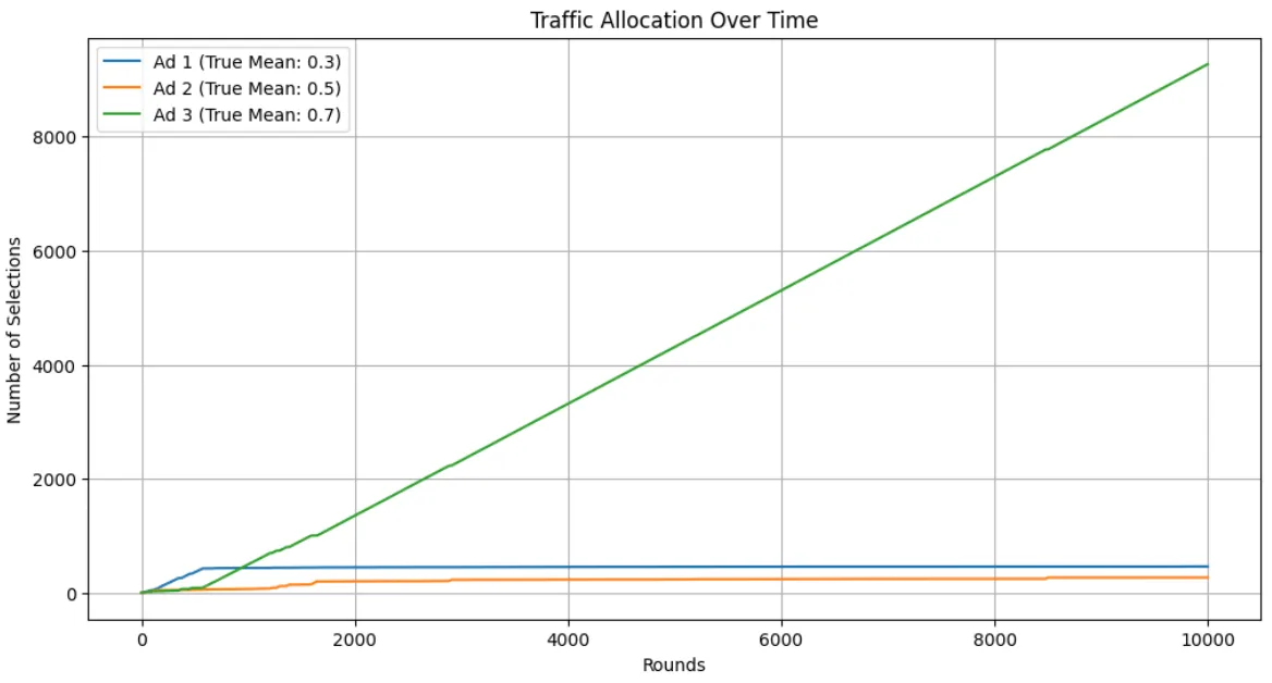
# Plot results
63
plt.figure(figsize=(12, 6))
64
for arm in range(bandit.n_arms):
65
    plt.plot(traffic_allocation[:, arm], label=f'Ad {arm+1} (True Mean: {true_mean_rewards[arm]})')
66
plt.title('Traffic Allocation Over Time')
67
plt.xlabel('Rounds')
68
plt.ylabel('Number of Selections')
69
plt.legend()
70
plt.grid()
71

72
# estimated
73
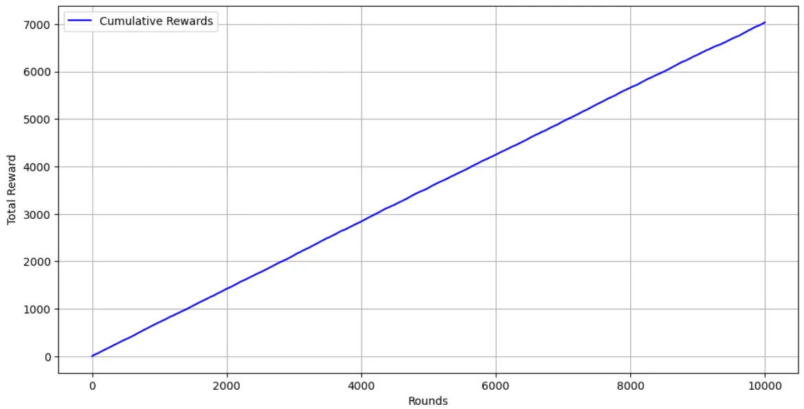
estimated_rewards = bandit.arm_rewards / (bandit.arm_counts + 1e-5)
74
plt.figure(figsize=(12,6))
75
plt.plot(range(n_rounds), cumulative_rewards, label='Cumulative Rewards', color='blue')
76
plt.xlabel('Rounds')
77
plt.ylabel('Total Reward')
78
plt.legend()
79
plt.grid()
80

81
# traffic allocation
82
plt.figure(figsize=(12,6))
83
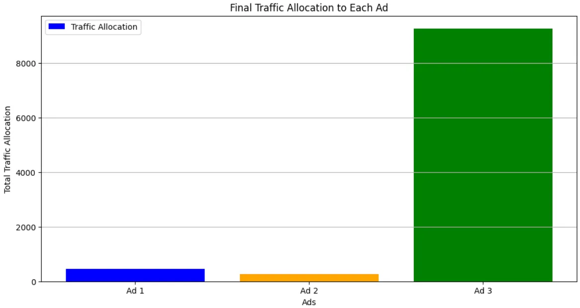
plt.bar(range(bandit.n_arms), traffic_allocation[-1], label='Traffic Allocation', color=['blue', 'orange', 'green'])
84
plt.xticks(range(bandit.n_arms), [f'Ad {i+1}' for i in range(bandit.n_arms)])
85
plt.title('Final Traffic Allocation to Each Ad')
86
plt.xlabel('Ads')
87
plt.ylabel('Total Traffic Allocation')
88
plt.legend()
89
plt.grid(True, axis='y')

Output

Thompson Sampling Implementation

Thompson Sampling is a Bayesian approach to the Multi-Armed Bandit problem that balances exploration and exploitation by sampling from the posterior distribution of each arm’s reward. It selects arms based on the probability that they are the best option, given the observed data.

Initialize prior distributions for each arm (e.g., Beta distribution for Bernoulli rewards).
For each round:
- Sample a reward probability from the posterior distribution of each arm.
- Select the arm with the highest sampled probability.
- Update the posterior distribution based on the observed reward.

1
import numpy as np
2
import matplotlib.pyplot as plt
3

4
np.random.seed(42)
5

6
# Epsilon-Greedy Bandit Algorithm
7
class SamplingBandit:
8
    def __init__(self, n_arms):
9
        self.n_arms = n_arms
10
        self.alpha = np.ones(n_arms)
11
        self.beta = np.ones(n_arms)
12
        self.arm_rewards = np.zeros(n_arms) # cumulative rewards for each arm
13
        self.arm_counts = np.zeros(n_arms)  # number of times each arm was pulled
14
        self.total_counts = 0               # total number of pulls
15

16
    def select_arm(self):
17
        sample_means = np.random.beta(self.alpha, self.beta)
18
        return np.argmax(sample_means)
19

20
    def update(self, arm, reward):
21
        self.arm_rewards[arm] += reward
22
        self.arm_counts[arm] += 1
23
        self.total_counts += 1
24
        if reward == 1: # reward observed
25
            self.alpha[arm] += 1
26
        else: # no reward
27
            self.beta[arm] += 1
28

29
# Simulation three ads with different reward distributions
30
true_mean_rewards = [0.3, 0.5, 0.7]
31
reward_distributions = [lambda: np.random.binomial(1, p) for p in true_mean_rewards]
32

33
# Parameters
34
n_arms = len(true_mean_rewards)
35
c = 1
36
delta_min = min(true_mean_rewards)
37

38
# Initialize bandit
39
bandit = SamplingBandit(n_arms)
40

41
# Run simulation
42
n_rounds = 10000
43
rewards = []
44
ad_selections = []
45
cumulative_rewards = np.zeros(n_rounds)
46
traffic_allocation = np.zeros((n_rounds, n_arms))
47

48
for t in range(n_rounds):
49
    selected_ad = bandit.select_arm()
50
    ad_selections.append(selected_ad)
51
    reward = reward_distributions[selected_ad]()
52
    rewards.append(reward)
53
    bandit.update(selected_ad, reward)
54
    cumulative_rewards[t] = cumulative_rewards[t-1] + reward if t > 0 else reward
55
    traffic_allocation[t] = bandit.arm_counts
56

57
# Plot results
58
plt.figure(figsize=(12, 6))
59
for arm in range(bandit.n_arms):
60
    plt.plot(traffic_allocation[:, arm], label=f'Ad {arm+1} (True Mean: {true_mean_rewards[arm]})')
61
plt.title('Traffic Allocation Over Time')
62
plt.xlabel('Rounds')
63
plt.ylabel('Number of Selections')
64
plt.legend()
65
plt.grid()
66

67
# estimated
68
estimated_rewards = bandit.arm_rewards / (bandit.arm_counts + 1e-5)
69
plt.figure(figsize=(12,6))
70
plt.plot(range(n_rounds), cumulative_rewards, label='Cumulative Rewards', color='blue')
71
plt.xlabel('Rounds')
72
plt.ylabel('Total Reward')
73
plt.legend()
74
plt.grid()
75

76
# traffic allocation
77
plt.figure(figsize=(12,6))
78
plt.bar(range(bandit.n_arms), traffic_allocation[-1], label='Traffic Allocation', color=['blue', 'orange', 'green'])
79
plt.xticks(range(bandit.n_arms), [f'Ad {i+1}' for i in range(bandit.n_arms)])
80
plt.title('Final Traffic Allocation to Each Ad')
81
plt.xlabel('Ads')
82
plt.ylabel('Total Traffic Allocation')
83
plt.legend()
84
plt.grid(True, axis='y')