Particle Swarm Optimization (PSO)

PSO is a population-based optimization technique inspired by the social behavior of birds flocking or fish schooling. Each particle represents a potential solution and adjusts its position based on its own experience and that of neighboring particles. It is also a metaheuristic algorithm.

Terminology

Particle: Represents a potential solution in the search space.
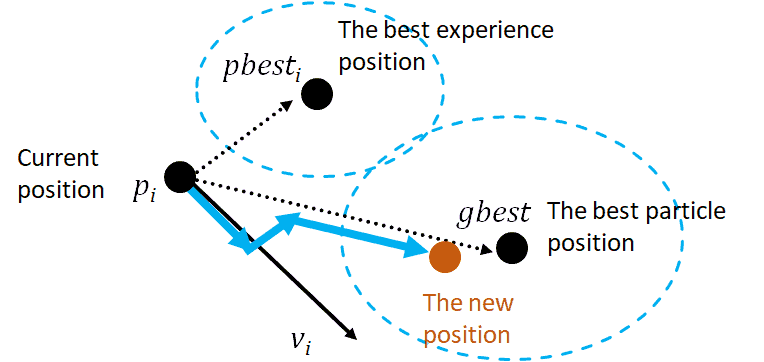
Velocity: The rate of change of the particle’s position.
- Defined by inertia, individual best, and swarm best.
Position: The current location of the particle in the search space.
Personal Best (pBest): The best position a particle has achieved so far.
Global Best (gBest): The best position achieved by any particle in the swarm.
Inertia Weight: A parameter that controls the impact of the previous velocity on the current velocity.

Algorithm Steps

Initialization
1. Initialize a population of particles with random positions and velocities.
2. Set the initial pBest for each particle to its starting position.
3. Set the initial gBest to the best pBest among all particles.
Velocity Update
1. Update the velocity of each particle based on its current velocity, the distance to its pBest, and the distance to the gBest.
2. The velocity update formula is given by:
  
  $v_{i}(t+1) = w \cdot v_{i}(t) + c_1 \cdot r_1 \cdot (pBest_{i} - x_{i}(t)) + c_2 \cdot r_2 \cdot (gBest - x_{i}(t))$
  where:
- $v_{i}(t)$ : Velocity of particle (i) at time (t)
- $x_{i}(t)$ : Position of particle (i) at time (t)
- $w$ : Inertia weight (controls the impact of the previous velocity)
- $c_1, c_2$ : Cognitive and social coefficients (control the influence of pBest and gBest)
- $r_1, r_2$ : Random numbers between 0 and 1
Position Update
1. Update the position of each particle based on its new velocity.
2. The position update formula is given by: $x_{i}(t+1) = x_{i}(t) + v_{i}(t+1)$
Fitness Evaluation
1. Evaluate the fitness of each particle’s new position using the objective function.
2. If the new position is better than the particle’s pBest, update pBest.
3. If the new pBest is better than the current gBest, update gBest.
Termination
1. Repeat steps 2-4 until a stopping criterion is met (e.g., a maximum number of iterations or a satisfactory fitness level).

Code Practice

Given Problem:

\max 40x + 30y \\ \text{s.t. } 2x + y \leq 100 \\ x + y \leq 80 \\ x \leq 40 \\ x, y \geq 0 \\

1
import numpy as np
2

3
def pso_LP(c, A, b,
4
           swarm_size=40, max_iter=200,
5
           w=0.75, c1=1.5, c2=1.5,
6
           penalty_scale=1e5):
7
    """
8
    Particle Swarm Optimization (PSO) for Linear Programs:
9
        max c^T x
10
        s.t. A x <= b, x >= 0
11

12
    Parameters
13
    ----------
14
    c : array_like
15
        Coefficients of the objective function (shape: n,)
16
    A : array_like
17
        Constraint matrix (shape: m, n)
18
    b : array_like
19
        RHS of constraints (shape: m,)
20
    swarm_size : int
21
        Number of particles
22
    max_iter : int
23
        Number of iterations
24
    w, c1, c2 : float
25
        Inertia, cognitive, and social coefficients
26
    penalty_scale : float
27
        Large penalty for constraint violations
28

29
    Returns
30
    -------
31
    gbest_position : ndarray
32
        Best solution found
33
    gbest_obj : float
34
        Objective value at best solution
35
    """
36

37
    # Convert inputs
38
    c = np.asarray(c, dtype=float).reshape(-1)
39
    A = np.asarray(A, dtype=float)
40
    b = np.asarray(b, dtype=float).reshape(-1)
41
    m, n = A.shape
42

43
    # Random initialization (x >= 0)
44
    pos = np.random.rand(swarm_size, n) * (b.max() / (A.max() + 1e-9))
45
    vel = np.random.randn(swarm_size, n)
46

47
    # Fitness evaluation
48
    def fitness(x):
49
        # objective
50
        obj = np.dot(c, x)
51
        # constraints violation (Ax <= b)
52
        violation = np.maximum(A @ x - b, 0.0)
53
        penalty = penalty_scale * violation.sum()
54
        return obj - penalty
55

56
    # Initialize personal bests
57
    pbest = pos.copy()
58
    pbest_val = np.array([fitness(x) for x in pos])
59

60
    # Initialize global best
61
    gbest_idx = np.argmax(pbest_val)
62
    gbest = pbest[gbest_idx].copy()
63
    gbest_val = pbest_val[gbest_idx]
64

65
    # Main loop
66
    for t in range(max_iter):
67
        for i in range(swarm_size):
68
            fval = fitness(pos[i])
69
            if fval > pbest_val[i]:
70
                pbest[i] = pos[i].copy()
71
                pbest_val[i] = fval
72

73
        # Update global best
74
        if np.max(pbest_val) > gbest_val:
75
            gbest_idx = np.argmax(pbest_val)
76
            gbest = pbest[gbest_idx].copy()
77
            gbest_val = pbest_val[gbest_idx]
78

79
        # Update velocities and positions
80
        r1, r2 = np.random.rand(swarm_size, n), np.random.rand(swarm_size, n)
81
        vel = (w * vel
82
               + c1 * r1 * (pbest - pos)
83
               + c2 * r2 * (gbest - pos))
84
        pos = pos + vel
85
        pos = np.clip(pos, 0, None)  # enforce x >= 0
86

87
    return gbest, gbest_val
88

89
# Define your problem
90
c = [40, 30]
91
A = [[2, 1],
92
     [1, 1],
93
     [1, 0]]
94
b = [100, 80, 40]
95

96
best_x, best_val = pso_LP(c, A, b)
97
print("Best solution (x, y):", best_x)
98
print("Objective value:", best_val)
99

100
# Output:
101
# Best solution (x, y): [19.99999995 59.99999999]
102
# Objective value: 2599.999997587528

Professor’s Code Version

This version is a little more robust, and has a stronger penalty for constraint violations.

1
import numpy as np
2

3
def pso_LP(c, A, b,
4
           swarm_size=40, max_iter=200,
5
           w=0.75, c1=1.5, c2=1.5,
6
           penalty_scale=1e5):
7
    """
8
    Particle Swarm Optimization (PSO) for LP:
9
        max c^T x  s.t.  A x <= b, x >= 0
10
    """
11

12
    # Convert inputs
13
    c = np.asarray(c, dtype=float).reshape(-1)
14
    A = np.asarray(A, dtype=float)
15
    b = np.asarray(b, dtype=float).reshape(-1)
16
    m, n = A.shape
17

18
    # Bounds [0, 80] (example upper bound; adjust if needed)
19
    bounds = [0, 80]
20

21
    # Initialize particles
22
    positions = np.random.uniform(low=bounds[0], high=bounds[1],
23
                                  size=(swarm_size, n))
24
    velocities = np.random.uniform(-0.05, 0.05, size=(swarm_size, n))
25

26
    # Penalized objective (we MINIMIZE)
27
    def penalized_obj(x_vec):
28
        base = -np.dot(c, x_vec)  # negate for maximization
29
        ineq_viol = np.maximum(0.0, np.dot(A, x_vec) - b)   # Ax <= b
30
        nonneg_viol = np.maximum(0.0, -x_vec)               # x >= 0
31
        penalty = penalty_scale * (np.sum(ineq_viol**2) + np.sum(nonneg_viol**2))
32
        return base + penalty
33

34
    # Personal and global bests
35
    pbest_positions = positions.copy()
36
    pbest_scores = np.array([penalized_obj(positions[i]) for i in range(swarm_size)])
37
    gbest_index = np.argmin(pbest_scores)
38
    gbest_position = pbest_positions[gbest_index].copy()
39
    gbest_score = float(pbest_scores[gbest_index])
40

41
    # Main loop
42
    for iteration in range(max_iter):
43
        for i in range(swarm_size):
44
            score = penalized_obj(positions[i])
45

46
            # Update personal best
47
            if score < pbest_scores[i]:
48
                pbest_scores[i] = score
49
                pbest_positions[i] = positions[i].copy()
50

51
            # Update global best
52
            if score < gbest_score:
53
                gbest_score = score
54
                gbest_position = positions[i].copy()
55

56
        # Update velocities and positions
57
        for i in range(swarm_size):
58
            r1, r2 = np.random.rand(n), np.random.rand(n)
59
            velocities[i] = (w * velocities[i]
60
                             + c1 * r1 * (pbest_positions[i] - positions[i])
61
                             + c2 * r2 * (gbest_position - positions[i]))
62
            positions[i] = positions[i] + velocities[i]
63
            # Keep inside bounds
64
            positions[i] = np.clip(positions[i], bounds[0], bounds[1])
65

66
    # Return best solution (convert back from minimized form)
67
    gbest_obj = float(np.dot(c, gbest_position))
68
    return gbest_position, gbest_obj
69

70
# Define your problem
71
c = [40, 30]
72
A = [[2, 1],
73
     [1, 1],
74
     [1, 0]]
75
b = [100, 80, 40]
76

77
best_x, best_val = pso_LP(c, A, b)
78
print("Best solution (x, y):", best_x)
79
print("Objective value:", best_val)
80

81
# Output:
82
# Best solution (x, y): [19.99995011 60.00014982]
83
# Objective value: 2600.0024989010058

HPO with PSO

This is the same problem solved with genetic algorithms in the previous lecture.

Given Problem:

\min_{\lambda} \ell(\theta, \omega^*; D_{val}) \\ \text{s.t. } 0 \leq \lambda \leq 1 \\ y(x) \in \text{argmin}_{\omega \in W} L(\omega; \lambda, D_{train}) \\

Use the following assumptions to generate the dataset:

True model: $y = 2x + 1$
$x$ : Generate 100 random $x$ values.
$y$ $y$ : Generate 100 $y$ $y$ values with the above $x$ $x$ and add error with a normal distribution.
- e.g. $y = 2x + 1 + \text{error}$
Use the same loss function on the upper and lower level.
- Ridge regression loss: $\Sigma (y - \hat{y})^2 + \lambda \times m^2, \text{where} \space \hat{y} = mx + b$

1
import numpy as np
2
from sklearn.linear_model import Ridge
3
from sklearn.model_selection import train_test_split
4
import matplotlib.pyplot as plt
5
import random
6

7
# Generate synthetic data
8
x = np.random.rand(100)
9
y = 2 * x + 1 + np.random.normal(0, 0.1, size=x.shape)
10

11
x_train, x_val, y_train, y_val = train_test_split(x, y, train_size=0.8)
12

13
# Lower-level: Ridge regression
14
def lower_opt(x_train, y_train, lambda_val):
15
    model = Ridge(alpha=lambda_val)
16
    model.fit(x_train, y_train)
17
    m = model.coef_
18
    b = model.intercept_
19
    return m, b
20

21
# Upper-level: Evaluate on validation set
22
def upper_eval(x_val, y_val, m, b, lambda_val):
23
    obj = sum((y_val[i] - (m * x_val[i] + b))**2 for i in range(len(y_val))) + lambda_val * m**2
24
    obj = obj[0]  # because sum returns numpy array w/ shape (1,)
25
    return obj
26

27
# PSO for HPO
28
def pso_HPO(x_train, y_train, x_val, y_val,
29
            swarm_size=20, max_iter=50,
30
            w=0.7, c1=1.5, c2=1.5):
31
    # Initialize particles (λ values between 0.0001 and 1)
32
    positions = np.random.uniform(0.0001, 1, size=swarm_size)
33
    velocities = np.random.uniform(-0.05, 0.05, size=swarm_size)
34

35
    # Personal and global bests
36
    personal_best_positions = positions.copy()
37
    personal_best_scores = np.full(swarm_size, np.inf)
38
    global_best_position = positions[0]
39
    global_best_score = np.inf
40

41
    for _ in range(max_iter):
42
        for i in range(swarm_size):
43
            m, b = lower_opt(x_train, y_train, positions[i])
44
            score = upper_eval(x_val, y_val, m, b, positions[i])
45

46
            # Update personal best
47
            if score < personal_best_scores[i]:
48
                personal_best_scores[i] = score
49
                personal_best_positions[i] = positions[i]
50

51
            # Update global best
52
            if score < global_best_score:
53
                global_best_score = score
54
                global_best_position = positions[i]
55

56
        # Update velocities and positions
57
        r1, r2 = np.random.rand(swarm_size), np.random.rand(swarm_size)
58
        velocities = (w * velocities
59
                      + c1 * r1 * (personal_best_positions - positions)
60
                      + c2 * r2 * (global_best_position - positions))
61
        positions += velocities
62

63
        # Keep λ within bounds [0.0001, 1]
64
        positions = np.clip(positions, 0.0001, 1)
65

66
    return global_best_position
67

68
# Run PSO for HPO
69
best_lambda_pso = pso_HPO(x_train.reshape(-1,1), y_train,
70
                          x_val.reshape(-1,1), y_val)
71

72
final_model = Ridge(alpha=best_lambda_pso)
73
final_model.fit(x_train.reshape(-1,1), y_train)
74

75
print(f"PSO 최적 λ: {best_lambda_pso:.4f}")
76

77
# Plot results
78
plt.scatter(x, y, color='blue', label='Data')
79
plt.plot(x, final_model.coef_ * x + final_model.intercept_,
80
         color='red', label=f'Ridge Regression (λ={best_lambda_pso:.4f})')
81
plt.xlabel('x')
82
plt.ylabel('y')
83
plt.title('Ridge Regression with PSO-optimized λ')
84
plt.legend()
85
plt.grid()
86
plt.show()