Forecasting Methods for Time Series

AR(p) Model

A linear forecasting model that uses past values to predict the current value.

X_t = a_0 + a_1 X_{t-1} + a_2 X_{t-2} + \ldots + a_p X_{t-p} + e_t

time series package: statsmodels
Regression with machine learning
- ex. multi-layer perceptron
- input layer — (hidden layers) —> output layer
$[X_{t-1}, X_{t-2}, \ldots, X_{t-p}] \rightarrow X_t$

Code Example

1
import numpy as np
2
import pandas as pd
3
import matplotlib.pyplot as plt
4
from statsmodels.tsa.ar_model import AutoReg
5
from statsmodels.graphics.tsaplots import plot_pacf, plot_acf
6

7
# Generate synthetic AR(2) data: daily CTR
8
np.random.seed(42)
9
n = 200
10
time = pd.date_range(start='2024-01-01', periods=n, freq='D')
11
ctr = np.sin(np.linspace(0,4*np.pi,n))*0.02 + 0.05 + np.random.normal(scale=0.005, size=n)
12

13
df = pd.DataFrame({'date': time, 'ctr': ctr})
14
df.set_index('date', inplace=True)
15

16
df['ctr'].plot(title='Daily CTR', figsize=(10, 4))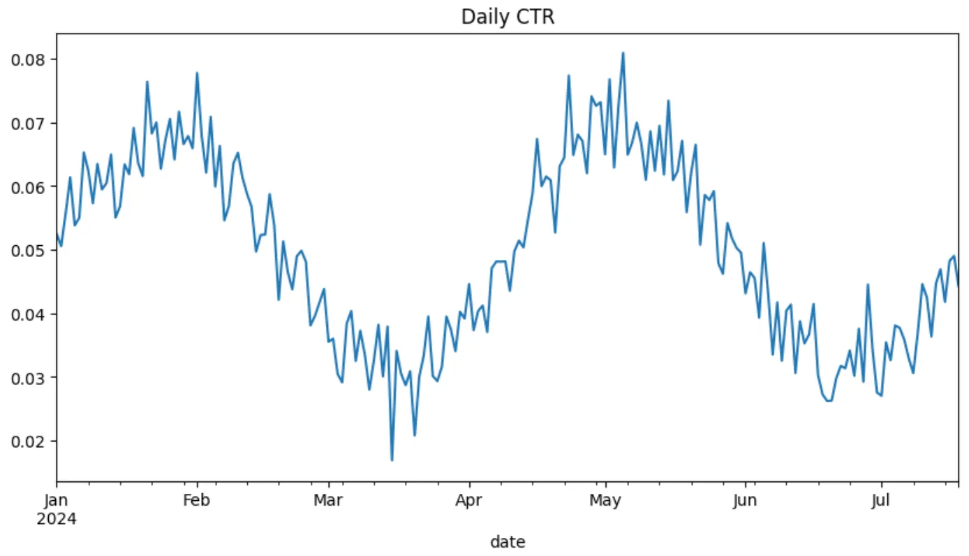
17
plt.show()

1
# Plot PACF
2
plot_acf(df['ctr'], lags=30)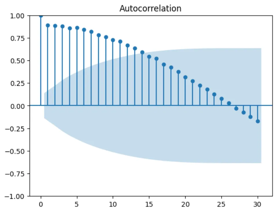
3
plt.show()

1
train_size = int(len(df) * 0.8)
2
train, test = df.iloc[:train_size], df.iloc[train_size:]
3

4
# Fit AR model
5
model = AutoReg(train['ctr'], lags=17)  # AR(17)
6
model_fit = model.fit()
7

8
# Make predictions
9
predictions = model_fit.predict(start=len(train), end=len(train)+len(test)-1, dynamic=False)
10

11
# Plot results
12
plt.figure(figsize=(10, 4))
13
plt.plot(train.index, train['ctr'], label='Train')
14
plt.plot(test.index, test['ctr'], label='Test')
15
plt.plot(test.index, predictions, label='Predictions', color='red')
16
plt.legend()
17
plt.title('AR Model Predictions')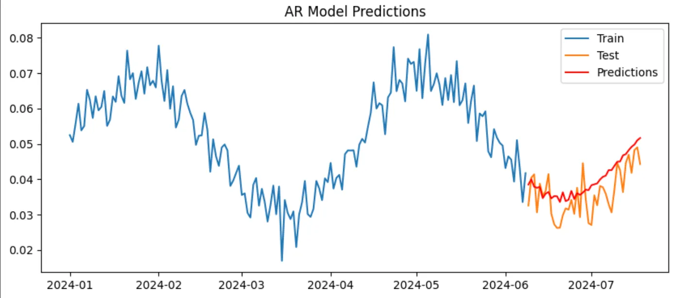
18
plt.show()

1
# exogenous variables (day of weeks)
2
exog = pd.get_dummies(df.index.dayofweek)
3
exog.columns = ['Mon', 'Tue', 'Wed', 'Thu', 'Fri', 'Sat', 'Sun']
4
exog.index = df.index
5

6
train_exog, test_exog = exog.iloc[:train_size], exog.iloc[train_size:]
7

8
# Fit AR model with exogenous variables
9
model_exog = AutoReg(train['ctr'], lags=17, exog=train_exog)
10
model_exog_fit = model_exog.fit()
11

12
# Make predictions with exogenous variables
13
predictions_exog = model_exog_fit.predict(start=len(train), end=len(train)+len(test)-1, exog_oos=test_exog, dynamic=False)
14

15
# Plot results
16
plt.figure(figsize=(10, 4))
17
plt.plot(train.index, train['ctr'], label='Train')
18
plt.plot(test.index, test['ctr'], label='Test')
19
plt.plot(test.index, predictions_exog, label='Predictions with Exog', color='green')
20
plt.legend()
21
plt.title('AR Model Predictions with Exogenous Variables')
22
plt.sh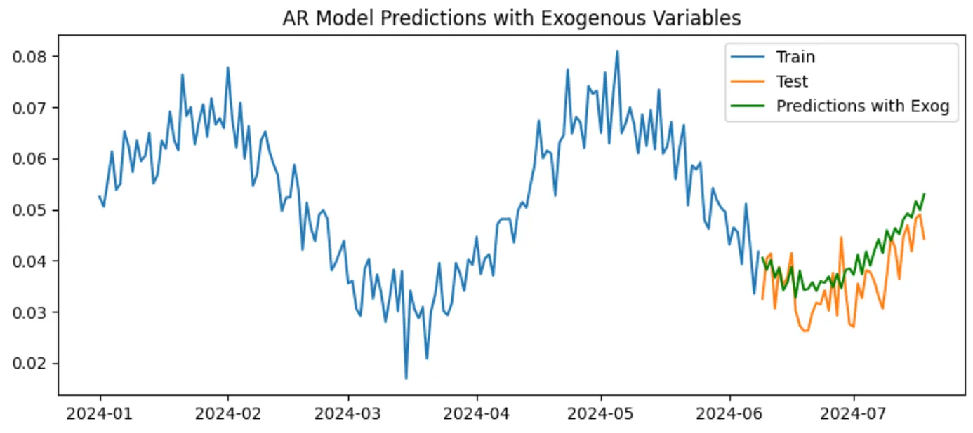ow()

Multi-Layer Perceptron (MLP) for Time Series

The goal is the find the weights that minimize the loss function (e.g., Mean Squared Error).

Structure:

Input layer: past values (lags)
Hidden layers: non-linear transformations
- Activation functions (ReLU, Sigmoid, Tanh):
  - ReLU: $f(x) = max(0, x)$
  - Sigmoid: $f(x) = \frac{1}{1 + e^{-x}}$
  - Tanh: $f(x) = \frac{e^x - e^{-x}}{e^x + e^{-x}}$
Output layer: predicted value

Training:

Forward pass: compute predictions
- Compute output: $\hat{y} = f(Wx + b)$ where $W$ are weights, $b$ is bias, and $f$ is activation function
- Compute loss: $L(y, \hat{y})$ (e.g., MSE: $L = \frac{1}{n} \sum (y_i -\hat{y}_i)^2$ )
Backward pass: compute gradients and update weights using optimization algorithms (e.g., SGD, Adam)
- This is known as backpropagation
- Compute gradients using chain rule
- Update weights: $w = w - \eta \nabla L(w)$ where $\eta$ is the learning rate and $\nabla L(w)$ is the gradient of the loss function with respect to weights
Repeat until convergence

Importance of lags

Note

There is a trade-off between historical information and total sample size!

For too many lags, the effective sample size decreases since we lose the first $p$ observations.

Lag determines the number of input nodes!

Lag—a hyperparameter—determines the input structure, the amount of historical information used to predict the current value, making it perhaps the most crucial hyperparameter in time series forecasting with MLPs.

Code Example

1
import numpy as np
2
import pandas as pd
3
import matplotlib.pyplot as plt
4

5
np.random.seed(42)
6

7
n = 365
8
time = pd.date_range(start='2023-01-01', periods=n, freq='D')
9
ctr = np.sin(np.linspace(0, 4 * np.pi, n)) * 0.02 + 0.05 + np.random.normal(scale=0.005, size=n)
10

11
df = pd.DataFrame({'date': time, 'ctr': ctr})
12

13
df.set_index('date', inplace=True)
14

15
df['ctr'].plot(title='Daily CTR', figsize=(10, 5))
16

17
plt.show()

1
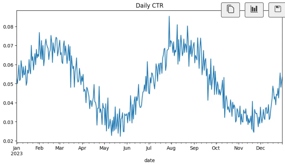
ctr_min = df['ctr'].min()
2
ctr_max = df['ctr'].max()
3

4
# normalization
5
df['ctr'] = (df['ctr'] - ctr_min) / (ctr_max - ctr_min)
6
df['ctr'].plot(figsize=(10, 5))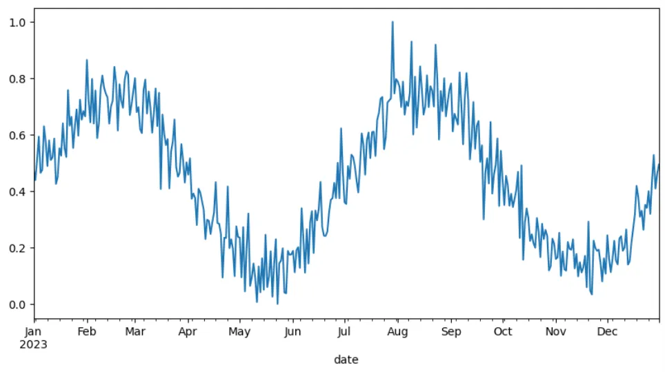

1
def create_lagged_data(series, lags=5):
2
    X, y = [], []
3
    for i in range(len(series)- lags):
4
        X.append(series[i:i+lags])
5
        y.append(series[i+lags])
6
    return np.array(X), np.array(y)
7

8
X_test, y_test = create_lagged_data(df['ctr'].values, lags=2)
9

10
for i in range(10):
11
    print(X_test[i], '->', y_test[i])
12

13
lags = 17
14
X, y = create_lagged_data(df['ctr'].values, lags=lags)
15

16
split = int(len(X) * 0.8)
17
X_train, y_train = X[:split], y[:split]
18
X_test, y_test = X[split:], y[split:]
19

20
train_dates = df.index[lags:split+lags]
21
test_dates = df.index[split+lags:]
22

23
# len(y_train), len(train_dates)
24

25
def intialize_weights(input_size, hidden_size, output_size):
26
    weights_input_hidden = np.random.uniform(-1, 1, (input_size, hidden_size))
27
    weights_hidden_output = np.random.uniform(-1, 1, (hidden_size, output_size))
28
    bias_hidden = np.random.uniform(-1, 1, (1, hidden_size,))
29
    bias_output = np.random.uniform(-1, 1, (1, output_size,))
30
    return weights_input_hidden, weights_hidden_output, bias_hidden, bias_output
31

32
def relu(x):
33
    return np.maximum(0, x)
34

35
def relu_derivative(x):
36
    return np.where(x > 0, 1, 0)
37

38
def mse_loss(y_true, y_pred):
39
    return np.mean((y_true - y_pred) ** 2)
40

41
def forward_pass(X, weights_input_hidden, weights_hidden_output, bias_hidden, bias_output):
42
    hidden_input = np.dot(X, weights_input_hidden) + bias_hidden
43
    hidden_output = relu(hidden_input)
44
    final_input = np.dot(hidden_output, weights_hidden_output) + bias_output
45
    final_output = final_input  # Linear activation for output layer
46
    return hidden_output, final_output
47

48
def backward_pass(X, y, hidden_output, final_output, weights_hidden_output):
49
    output_error = final_output - y # 교수님은 y - final_output으로 하긴 함,,
50
    output_delta = output_error  # Derivative of linear activation is 1
51

52
    hidden_error = np.dot(output_delta, weights_hidden_output.T) # *2 in class
53
    hidden_delta = hidden_error * relu_derivative(hidden_output)
54

55
    return output_delta, hidden_delta
56

57
def update_weights(X, hidden_output, output_delta, hidden_delta, weights_input_hidden, weights_hidden_output, bias_hidden, bias_output, learning_rate):
58
    weights_hidden_output -= np.dot(hidden_output.T, output_delta) * learning_rate
59
    weights_input_hidden -= np.dot(X.T, hidden_delta) * learning_rate
60
    bias_output -= np.sum(output_delta, axis=0, keepdims=True) * learning_rate
61
    bias_hidden -= np.sum(hidden_delta, axis=0, keepdims=True) * learning_rate
62
    return weights_input_hidden, weights_hidden_output, bias_hidden, bias_output
63

64
def train_mlp(X, y, input_size, hidden_size, output_size, epochs=1000, learning_rate=0.001):
65
    weights_input_hidden, weights_hidden_output, bias_hidden, bias_output = intialize_weights(input_size, hidden_size, output_size)
66

67
    for epoch in range(epochs):
68
        hidden_output, final_output = forward_pass(X, weights_input_hidden, weights_hidden_output, bias_hidden, bias_output)
69

70
        loss = mse_loss(y, final_output)
71

72
        output_delta, hidden_delta = backward_pass(X, y, hidden_output, final_output, weights_hidden_output)
73

74
        weights_input_hidden, weights_hidden_output, bias_hidden, bias_output = update_weights(X, hidden_output, output_delta, hidden_delta, weights_input_hidden, weights_hidden_output, bias_hidden, bias_output, learning_rate)
75

76
        if epoch % 100 == 0:
77
            print(f'Epoch {epoch}, Loss: {loss}')
78

79
    return weights_input_hidden, weights_hidden_output, bias_hidden, bias_output
80

81
def predict(X, weights_input_hidden, weights_hidden_output, bias_hidden, bias_output):
82
    _, final_output = forward_pass(X, weights_input_hidden, weights_hidden_output, bias_hidden, bias_output)
83
    return final_output
84

85
input_size = lags
86
hidden_size = 10
87
output_size = 1
88
weights_input_hidden, weights_hidden_output, bias_hidden, bias_output = train_mlp(X_train, y_train.reshape(-1, 1), input_size, hidden_size, output_size, epochs=1000, learning_rate=0.001)
89

90
predictions = predict(X_test, weights_input_hidden, weights_hidden_output, bias_hidden, bias_output)
91
predictions = predictions.flatten()
92
y_test = y_test.flatten()

Output:

1
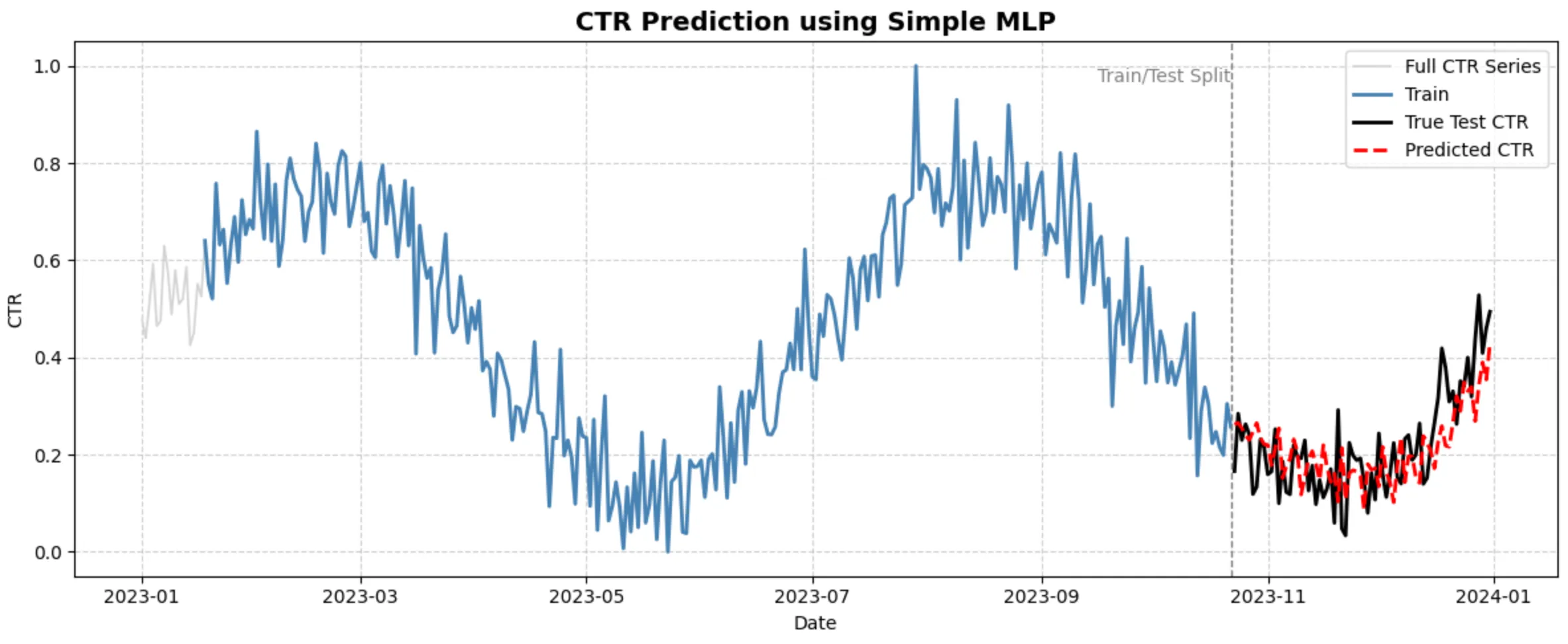
Epoch 0, Loss: 5.632162843223016
2
Epoch 100, Loss: 0.05115925220822442
3
Epoch 200, Loss: 0.04275551312820102
4
Epoch 300, Loss: 0.02245051661551441
5
Epoch 400, Loss: 0.018830809997783342
6
Epoch 500, Loss: 0.016457206995812355
7
Epoch 600, Loss: 0.014710278047137417
8
Epoch 700, Loss: 0.013191127588598398
9
Epoch 800, Loss: 0.012093276219005963
10
Epoch 900, Loss: 0.011152334762943965

1
plt.figure(figsize=(12, 5))
2
plt.plot(df.index, df['ctr'], color='lightgray', label='Full CTR Series', linewidth=1.2)
3
plt.plot(train_dates, y_train, color='steelblue', label='Train', linewidth=2)
4
plt.plot(test_dates, y_test, color='black', label='True Test CTR', linewidth=2)
5
plt.plot(test_dates, predictions, color='red', linestyle='--', label='Predicted CTR', linewidth=2)
6

7
plt.axvline(x=train_dates[-1], color='gray', linestyle='--', linewidth=1)
8
plt.text(train_dates[-1], plt.ylim()[1]*0.95, 'Train/Test Split', ha='right', va='top', fontsize=10, color='gray')
9

10
plt.title('CTR Prediction using Simple MLP', fontsize=14, weight='bold')
11
plt.xlabel('Date')
12
plt.ylabel('CTR')
13
plt.grid(True, linestyle='--', alpha=0.6)
14
plt.legend()
15
plt.tight_layout()
16
plt.show()