S-Curve Transformation

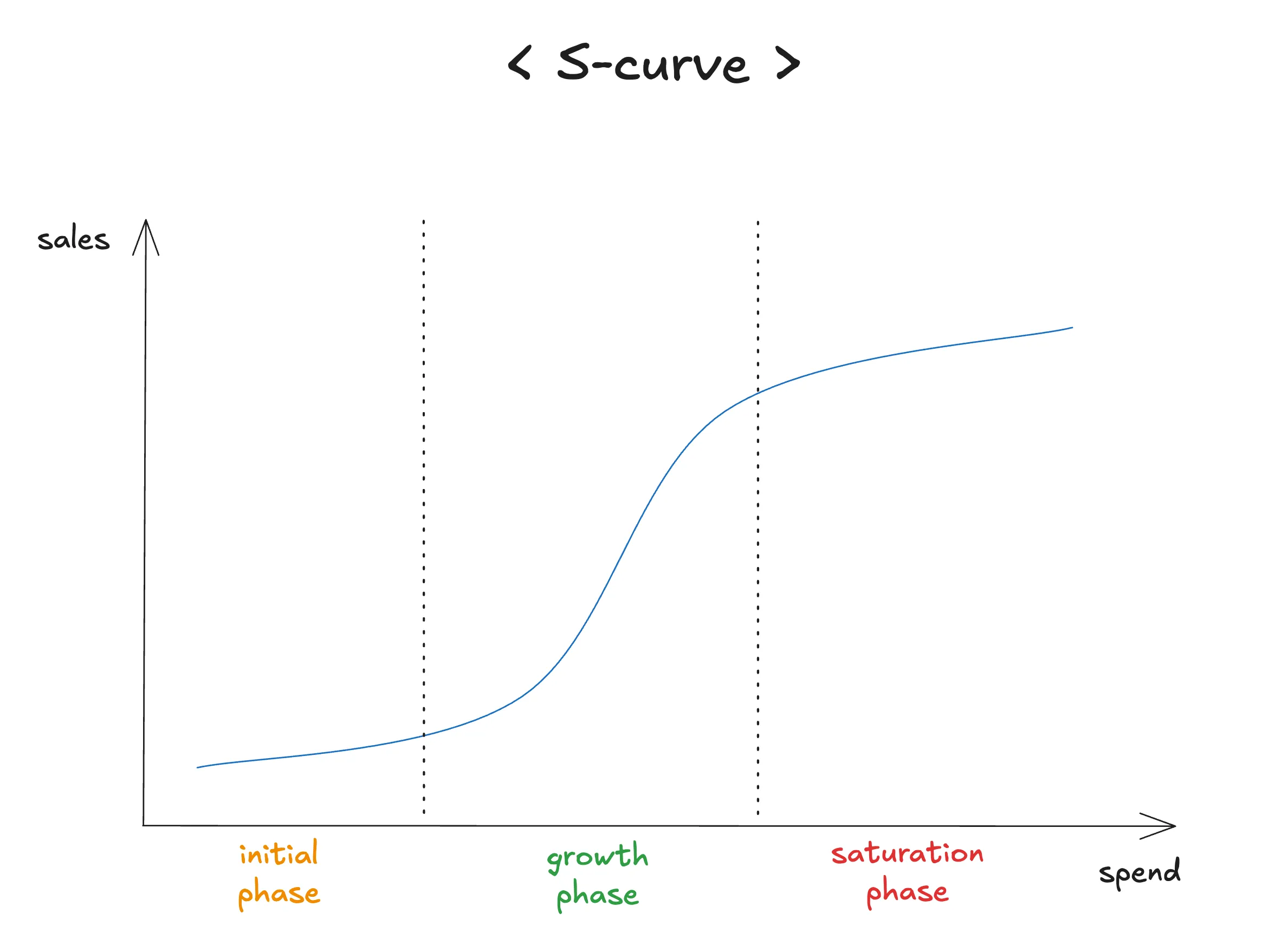
The S-Curve is the core concept that explains the non-linear relationship between advertising spend and performance outcomes (such as revenue or conversions). Unlike the simplistic assumption that “doubling ad spend will double sales,” the S-Curve reflects the Law of Diminishing Returns commonly observed in marketing. In other words, once advertising spend passes a certain point, efficiency gradually declines, and each additional dollar yields less impact.

In Marketing Mix Modeling (MMM), S-Curves are typically modeled using mathematical functions such as the logistic function or the Hill function, which allow analysts to statistically estimate the curve and calculate channel-specific parameters that define its shape.

Key Phases of the S-Curve

1. Ramp-up Phase (Gradual Growth)

• Position on curve: Lower section of the S-shape.
• Characteristics: This is the early stage of ad spending, where brand or message exposure is still limited. As a result, performance does not increase proportionally with spend, since consumers need repeated exposure and time before reacting.
• ROI: Relatively low. Spend may appear inefficient in this phase.
• Implication: There is a threshold effect—too little budget produces no meaningful impact and risks being wasted.

2. Sweet Spot / Steep Growth Phase

• Position on curve: Middle, steepest section of the S-shape.
• Characteristics: The “optimal efficiency zone,” where ad effects accelerate rapidly. Once exposure surpasses the threshold, even modest increases in spend drive disproportionately large performance gains. Brand awareness surges and conversions grow quickly.
• ROI: Highest in this phase. This is the ideal target range for budget allocation.
• Implication: A key objective in MMM is to identify this “sweet spot” for each channel and concentrate spend there.

3. Saturation / Plateau Phase

• Position on curve: Upper, flattening section of the S-shape.
• Characteristics: At high levels of spend, the market becomes saturated. Most target customers have already been reached, or ad fatigue sets in. Additional spend produces minimal incremental impact.
• ROI: Declines sharply. Further investment is inefficient and risks waste.
• Implication: When a channel reaches this phase, budgets should be cut back and reallocated to other channels that are still in the growth phase.

S-Curve Code Implementation Example

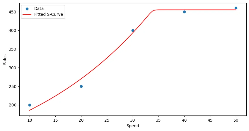
• A is the maximum possible sales (plateau).
• B controls the growth rate.
• C is the inflection point (where sales increase quickly).

1
import numpy as np
2
import pandas as pd
3
import matplotlib.pyplot as plt
4
from scipy.optimize import curve_fit
5

6
# create dataset
7
data = {
8
   'Day' : ['Mon', 'Tue', 'Wed', 'Thu', 'Fri'],
9
   'Spend' : [10, 20, 30, 40, 50],
10
   'Sales' : [200, 250, 400, 450, 460]
11
}
12
df = pd.DataFrame(data)
13

14
# define s-curve function
15
x_data = df['Spend']
16
y_data = df['Sales']
17
def s_curve(x, A, B, C):
18
   return A / (1 + np.exp(-B * (x - C)))
19

20
optimal_params, covariance = curve_fit(
21
   s_curve,
22
   x_data,
23
   y_data,
24
   p0=[max(y_data), 0.1, np.median(x_data)] # initial point (A, B, C)
25
)
26

27
A, B, C = optimal_params
28
print(f"Optimal parameters: A={A}, B={B}, C={C}")
29
# Optimal parameters: A=501.0309931841163, B=0.0844223122026954, C=16.67591505186686
30

31
# plot results
32
x_fit = np.linspace(min(x_data), max(x_data), 100)
33
y_fit = s_curve(x_fit, *optimal_params)
34
plt.scatter(x_data, y_data, label='Data')
35
plt.plot(x_fit, y_fit, color='red', label='Fitted S-Curve')
36
plt.xlabel('Spend')
37
plt.ylabel('Sales')
38
plt.legend()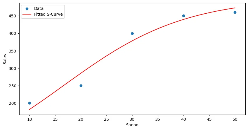

Generalized S-Curve (Richards’ Curve)

• $A$: Plateau; maximum sales
• $B$: Growth rate
• $C$: Inflection point
• $v$: Asymmetry parameter

if $v=1$, same as basic logistic function.
if $v<1$, slow early growth, rapid later growth.
if $v>1$, rapid early growth, slow later growth.

code implementation example:

1
import numpy as np
2
import pandas as pd
3
import matplotlib.pyplot as plt
4
from scipy.optimize import curve_fit
5

6
# create dataset
7
data = {
8
   'Day' : ['Mon', 'Tue', 'Wed', 'Thu', 'Fri'],
9
   'Spend' : [10, 20, 30, 40, 50],
10
   'Sales' : [200, 250, 400, 450, 460]
11
}
12
df = pd.DataFrame(data)
13

14
# define s-curve function
15
x_data = df['Spend']
16
y_data = df['Sales']
17
def s_curve(x, A, B, C, nu=1):
18
   return A * (1 + nu*np.exp(-B * (x - C)))**(-1/nu)
19

20
optimal_params, covariance = curve_fit(
21
   s_curve,
22
   x_data,
23
   y_data,
24
   p0=[max(y_data), 0.1, np.median(x_data), 0.9] # initial point (A, B, C, nu)
25
)
26

27
A, B, C, nu = optimal_params
28
print(f"Optimal parameters: A={A}, B={B}, C={C}, nu={nu}")
29
# Optimal parameters: A=455.0000003735234, B=4.078058186448524, C=32.74072510361706, nu=108.54222404122513
30

31
# plot results
32
x_fit = np.linspace(min(x_data), max(x_data), 100)
33
y_fit = s_curve(x_fit, *optimal_params)
34
plt.scatter(x_data, y_data, label='Data')
35
plt.plot(x_fit, y_fit, color='red', label='Fitted S-Curve')
36
plt.xlabel('Spend')
37
plt.ylabel('Sales')
38
plt.legend()