Hyperparameter Optimization

Model Parameter

• Configuration variable that is internal to the model and whose value can be estimated from data.
• e.g., weights in linear regression, weights and biases in neural networks.

Characteristics

• They are required by the model when making predictions.
• They values define the skill of the model on your problem.
• They are estimated or learned from data.
• They are often not set manually by the practitioner.
• They are often saved as part of the learned model.

Hyperparameter

• Configuration variable that is external to the model and whose value cannot be estimated from data.
• e.g., learning rate, number of hidden layers, number of clusters.

Characteristics

• They are often used in the process to help estimate model parameters.
• They can often be set using heuristics.
• They are often tuned for a given predictive modeling problem.

Bilevel optimization

Bi-level Optimization has a nested structure where one optimization problem is contained within another. It consists of an upper-level problem and a lower-level problem, with the solution of the upper-level problem depending on the solution of the lower-level problem.

• $\theta$: Hyperparameter. The variable we want to optimize (e.g., learning rate, number of hidden units, regularization strength).
• $\Omega$: The search space where the hyperparameter $\theta$ can exist.
• $w$: Model Parameter. The values that the model learns through training (e.g., weights and biases of a neural network).
• $D = (D_{\text{train}}, D_{\text{val}})$: The dataset, split into
  • $D_{\text{train}}$: Data used to train the model parameters $w$.
  • $D_{\text{val}}$: Data used to (1) evaluate the generalization performance of the trained model and (2) to find the optimal hyperparameter $\theta$.
• $L$: Training loss function. The criterion used to optimize $w$ during training, measuring how well the model predicts $D_{\text{train}}$.
• $\ell$: Validation loss function. The criterion used to evaluate the quality of the hyperparameter $\theta$, measuring how well the model trained on $D_{\text{train}}$ performs on unseen data $D_{\text{val}}$.

Example

1. Select a feasible hyperparameter $\theta$ from the search space $\Omega = [-5, 5]$. For example, let $\theta = 3$.
2. Solve the lower-level problem to find the optimal model parameter $w^*$ given the hyperparameter $\theta = 3$.
   • solve $min(\theta - w)^2$ with respect to $w$.
   • The lower-level problem is to minimize the training loss $L(\theta, w) = (3 - w)^2$ with respect to $w$.
   • The optimal solution is $w^* = 3$.
3. Evaluate the upper-level objective function $\ell(\theta, w^*)$ using the obtained $w^*$.
   • The upper-level problem is to minimize the validation loss $\ell(\theta, w^*) = \theta^2 + (w^*)^2$.
   • Substituting $\theta = 3$ and $w^* = 3$, we get $\ell(3, 3) = 3^2 + 3^2 = 18$.

Using Grid Search

Grid Search is a method for finding the optimal hyperparameters by exhaustively trying all possible combinations based on a predefined grid of hyperparameter values.

• Most basic hyperparameter optimization method.
• Full factorial design
  • Evaluates all possible combinations of hyperparameters.
  • Guarantees finding the global optimum if given enough resources.
  • curse of dimensionality: Computational cost increases exponentially with the number of hyperparameters.

It is the cartesian product of hyperparameter values.

Using Random Search

When iterations are limited, each trial has the opportunity to explore new values for each hyperparameter, increasing the chances of finding the optimal values for the important parameters.

Random Search is a method for finding the optimal hyperparameters by randomly sampling combinations of hyperparameter values from predefined ranges.

• Works better than Grid Search when some hyperparameters are more important than others. (Which is true in most cases)
• But you don’t know how many samples you need to draw to find a good combination.

Bi-level Black-Box Optimization Problem

Black-box optimization methods obtain the optimal results without needing to understand the internal mechanics.

• The overall shape of the upper-level objective function $\ell(\theta)$ is unknown.
• Derivative-free optimization method: gradients and hessians are not needed.

Common Black-Box Optimization Methods

• Bayesian Optimization:
  • Builds a probabilistic model of the objective function and uses it to select the most promising hyperparameters to evaluate next.
  • This can be considered as a surrogate-based derivative-free optimization algorithm.
• Evolutionary Algorithms:
  • Mimics the process of natural selection to evolve a population of candidate solutions. (aka. Genetic Algorithms)
• Random Search:
  • Randomly samples hyperparameter combinations from predefined distributions.
• Surrogate-based Derivative-Free Optimization Algorithms:
  • Uses a surrogate model to approximate the objective function and guide the search for optimal hyperparameters.

Surrogate-based Derivative-Free Optimization Algorithm in Hyperparameter Optimization

1. Prepare hyperparameters for optimization

   • Map the finite set of possible values using sequences of integers.
   • Domain denoted as $\Omega$.

2. Initial design

   • Create an initial experimental design with $n_0$ samples by random sampling from $\Omega$.
   • For each sampled candidate $\theta_j \in \Omega$, compute the upper level objective function value ($\ell(\theta_j)$) by solving the lower-level problem
   • e.g., training and validating a model with hyperparameter $\theta_j$.

3. Set $n \leftarrow n_0$

   • Record the number of evaluations.

4. Adaptive sampling

   • Iteratively select new candidates $\theta^{new}$ to evaluate based on previous results.

5. Surrogate model fitting

   • Use the data $(\theta_j, \ell(\theta_j))$ obtained so far to fit a surrogate model.
   • This surrogate model is a cheaper approximation of the expensive objective function.
   • methods:
     • Gaussian Processes (GP): Probabilistic model that provides uncertainty estimates.
     • Radial Basis Functions (RBF): Approximate response surface of the objective function.

6. Acquisition function optimization

   • Optimize the acquisition function using the surrogate model.
   • This optimization process identifies the most promising candidate $\theta^{new}$ to evaluate next.
   • Exploration vs. Exploitation trade-off:
     • Exploration: Searching new areas of the hyperparameter space.
     • Exploitation: Focusing on areas known to yield good results.

7. Lower-level problem solving

   • Solve the lower-level problem for the newly selected hyperparameter $\theta^{new}$.
   • Obtain the objective function value $\ell(\theta^{new})$.

8. Update

   • Update $n \leftarrow n + 1$
   • Go back to Step 5.

9. Stopping criterion

   • Stop if the termination condition is met.
   • e.g.: max number of evaluations, time budget, convergence criteria.

Code Practice

Bilevel Optimization with Random search

1
import random
2
import pyomo.environ as pyo
3
import numpy as np
4
import matplotlib.pyplot as plt
5

6
random.seed(21)
7

8
# lower level problem solve for y given x
9
def solve_lower_level(x):
10
    model = pyo.ConcreteModel()
11
    model.y = pyo.Var(within=pyo.NonNegativeReals, bounds=(0, x))
12
    model.obj = pyo.Objective(expr=(model.y - 5)**2, sense=pyo.minimize)
13

14
    solver = pyo.SolverFactory('ipopt')
15
    solver.solve(model)
16
    return model.y.value
17

18
# evaluate upper level optimization problem
19
def evaluate_upper_level(x, y):
20
    return x**2 + y**2
21

22
# test functions
23
for i in [0, 5, 10]:
24
    print(f"Optimal y for x={i}: {solve_lower_level(i)}")
25

26
for i in [0, 5, 10]:
27
    print(f"Upper level objective for x={i}, y={solve_lower_level(i)}: {evaluate_upper_level(i, solve_lower_level(i))}")
28

29
# iterate randomly to find optimal x, y
30
def upper_level_random_search(num_iterations=1000):
31
    best_x = None
32
    best_y = None
33
    min_objective_value = float('inf')
34

35
    for i in range(num_iterations):
36
        x_candidate = random.uniform(0, 10)
37
        y_candidate = solve_lower_level(x_candidate)
38
        objective_value = evaluate_upper_level(x_candidate, y_candidate)
39

40
        if objective_value < min_objective_value:
41
            min_objective_value = objective_value
42
            best_x = x_candidate
43
            best_y = y_candidate
44
            print(f"Iteration {i+1}: New best found -> x = {best_x:.4f}, y = {best_y:.4f}, f(x,y) = {min_objective_value:.4f}")
45

46
    print("\nOptimal solution:")
47
    print(f"  x = {best_x:.4f}")
48
    print(f"  y = {best_y:.4f}")
49
    print(f"  Minimum f(x, y) = {min_objective_value:.4f}")
50

51
    return best_x, best_y, min_objective_value
52

53
upper_level_random_search()

Output:

1
Iteration 1: New best found -> x = 1.6495, y = 1.6495, f(x,y) = 5.4417
2
Iteration 11: New best found -> x = 0.0318, y = 0.0318, f(x,y) = 0.0020
3

4
Optimal solution:
5
  x = 0.0318
6
  y = 0.0318
7
  Minimum f(x, y) = 0.0020

Visualization

1
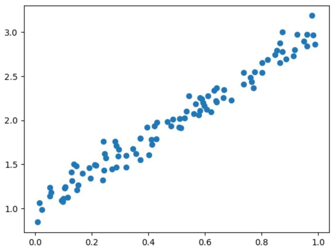
# generate data
2
x = np.random.rand(100)
3
y = 2 * x + 1 + np.random.normal(0, 0.1, 100)  # y = 2x + 1 + noise
4
plt.scatter(x, y)
5

6
# split data
7
split_index = int(0.8 * len(x))
8
x_train, x_val = x[:split_index], x[split_index:]
9
y_train, y_val = y[:split_index], y[split_index:]

Output:

Hyperparameter Optimization with Random Search

Use the following assumptions to generate the dataset:

• True model: $y = 2x + 1$
• $x$: Generate 100 random $x$ values.
• $y$: Generate 100 $y$ values with the above $x$ and add error with a normal distribution.
  • e.g. $y = 2x + 1 + \text{error}$
• Use the same loss function on the upper and lower level.
  • Ridge regression loss: $\Sigma (y - \hat{y})^2 + \lambda \times m^2, \text{where} \space \hat{y} = mx + b$

1
def solve_lower_level(lambda_value, x_train, y_train):
2
    model = pyo.ConcreteModel()
3
    model.m = pyo.Var(within=pyo.Reals)
4
    model.b = pyo.Var(within=pyo.Reals)
5

6
    def obj_func(model):
7
        return sum((y_train[i] - (model.m * x_train[i] + model.b))**2 for i in range(len(x_train))) + lambda_value * (model.m**2)
8
    model.obj = pyo.Objective(expr=obj_func(model), sense=pyo.minimize)
9

10
    solver = pyo.SolverFactory('ipopt')
11
    solver.solve(model)
12
    return model.m.value, model.b.value
13

14
solve_lower_level(0.1, x_train, y_train)
15
# Output: (1.9602579300437144, 1.013876477469167)
16

17
def upper_level_random_search(num_iterations=1000):
18
    best_lambda = None
19
    best_m = None
20
    best_b = None
21
    min_val_loss = float('inf')
22

23
    for i in range(num_iterations):
24
        lambda_candidate = random.uniform(0, 1)
25
        m_candidate, b_candidate = solve_lower_level(lambda_candidate, x_train, y_train)
26
        val_loss = np.mean([(y_val[j] - (m_candidate * x_val[j] + b_candidate))**2 for j in range(len(x_val))])  + lambda_candidate * (m_candidate**2)
27

28
        if val_loss < min_val_loss:
29
            min_val_loss = val_loss
30
            best_lambda = lambda_candidate
31
            best_m = m_candidate
32
            best_b = b_candidate
33
            print(f"Iteration {i+1}: New best -> λ = {best_lambda:.4f}, m = {best_m:.4f}, b = {best_b:.4f}, Val Loss = {min_val_loss:.4f}")
34

35
    print("\nOptimal solution:")
36
    print(f"  lambda = {best_lambda:.4f}")
37
    print(f"  m = {best_m:.4f}")
38
    print(f"  b = {best_b:.4f}")
39
    print(f"  Minimum Validation Loss = {min_val_loss:.4f}")
40

41
    return best_lambda, best_m, best_b, min_val_loss
42

43
upper_level_random_search()

Output:

1
Iteration 1: New best -> λ = 0.4744, m = 1.8421, b = 1.0714, Val Loss = 1.6210
2
Iteration 3: New best -> λ = 0.2508, m = 1.9109, b = 1.0379, Val Loss = 0.9258
3
Iteration 7: New best -> λ = 0.2438, m = 1.9131, b = 1.0368, Val Loss = 0.9022
4
Iteration 9: New best -> λ = 0.2171, m = 1.9217, b = 1.0327, Val Loss = 0.8117
5
Iteration 10: New best -> λ = 0.1569, m = 1.9413, b = 1.0231, Val Loss = 0.6010
6
Iteration 20: New best -> λ = 0.1438, m = 1.9456, b = 1.0210, Val Loss = 0.5542
7
Iteration 22: New best -> λ = 0.0404, m = 1.9805, b = 1.0040, Val Loss = 0.1681
8
Iteration 54: New best -> λ = 0.0089, m = 1.9913, b = 0.9987, Val Loss = 0.0452
9
Iteration 119: New best -> λ = 0.0001, m = 1.9944, b = 0.9973, Val Loss = 0.0103
10

11
Optimal solution:
12
  lambda = 0.0001
13
  m = 1.9944
14
  b = 0.9973
15
  Minimum Validation Loss = 0.0103