Stochastic Process
A stochastic process is a collection of random variables representing the evolution of some system of random values over time.
A sequence of random variables
is called a stochastic process, where is countable/uncountable set, often representing time, and is the sample path.
Example: Markov Chain (Markov Decision Process)
Note
- Random variable is when only random variable is considered.
- Stochastic process is when both time and random variable are considered.
이건 확랜프 참고 하삼
Discrete-Time Markov Chain (DTMC)
A discrete-time Markov chain is a stochastic process that satisfies the Markov property and evolves in discrete time steps.
A stochastic process in discrete time
If we write : means the system is in state at time .
Example: Consecutive coin tossing
- : number of heads in tosses
- Sample space: —> these are the states?
Basic Properties of DTMC
-
A Discrete Index Set
- This typically is the “time” index.
-
A Countable State Space
- Denoted by . Contains the possible states that can take.
- Can be finite or countably infinite.
-
The Markov Property
- The Markov property states that the future state depends only on the current state and not on the sequence of events that preceded it.
- Only depends on current time , and not on the past states .
- In other words, the next state only depends on the current state.
This is the probability that the system transitions into state at time given that it is in state at time .
Chapman-Kolmogorov Equations
(transition probability matrix) is a square matrix where the element at row and column represents the probability of transitioning from state to state in one time step. It has entries
Now, the m-step transition probability is defined as
The Chapman-Kolmogorov equations relate the m-step transition probabilities to the one-step transition probabilities. They state that the probability of transitioning from state to state in steps can be computed by summing over all possible intermediate states after steps:
for all and all states .
By the Chapman-Kolmogorov equations, we are performing matrix multiplication of the transition probability matrix .
Example: Weather Chains
Example (Weather Chain): Suppose if it is rainy or snowy in Suwon today, the probability that it will rain or snow tomorrow is 40%. If, on the other hand, if it is sunny in Suwon today, the probability that it will rain or snow tomorrow is 70%. Let
- State 0 := Rainy/Snowy
- State 1 := Sunny
Draw the state transition diagram of Suwon’s weather DTMC.
This gives us the transition probability matrix
We can compute the two-step transition probability matrix by squaring the one-step transition probability matrix:
What if we wanted to look at days 4, 8, and 16?
We can compute this by continuing to square the matrix:
Code Example
import numpy as np
P = np.array([[0.4, 0.6], [0.7, 0.3]])
P2 = np.matmul(P, P)
P4 = np.matmul(P2, P2)
P8 = np.matmul(P4, P4)
P16 = np.matmul(P8, P8)Output
As we can see, as we continue to square the matrix, the rows of the resulting matrix converge to the same values. This indicates that the Markov chain is reaching a steady state, where the probabilities of being in each state stabilize over time. This is called the steady-state distribution.
Mathematically,
This limit exists and is the same for all for a fixed state .
Example: Smart Phone Brand Preference
There are 3 categories of smart phone brands: iPhone, Android, or Windows Mobile. Customers who buy their nth smart phone in one of these brands, prefer the same brand for their next phone purchase with probability 0.8, 0.6, or 0.4, respectively. When they change their brand, they do so randomly among the remaining two brands. Find the long-run proportion of time a customer will have an iPhone, Android, or a Windows Mobile phone.
Let 0 := iPhone, 1 := Android, 2 := Windows Mobile.
Code Example
import numpy as np
P = np.array([[0.8, 0.1, 0.1], [0.2, 0.6, 0.2], [0.3, 0.3, 0.4]])P2 = np.matmul(P, P)P4 = np.matmul(P2, P2)P8 = np.matmul(P4, P4)P16 = np.matmul(P8, P8)P32 = np.matmul(P16, P16)Output
Now we need to solve for the steady-state distribution .
from scipy.linalg import solve
pi1, pi2, pi3 = symbols('pi1 pi2 pi3')
system = [ Eq(pi1, 0.8 * pi1 + 0.2 * pi2 + 0.3 * pi3), Eq(pi2, 0.1 * pi1 + 0.6 * pi2 + 0.3 * pi3), Eq(pi1 + pi2 + pi3, 1)]
solution = solve(system, (pi1, pi2, pi3))solutionOutput
{pil: 0.545454545454545, pi2: 0.272727272727273, pi3: 0.181818181818182}Google PageRank Algorithm
The Google PageRank algorithm measures the importance of web pages based on their link structure. That is, instead of counting links coming from different pages equally, we normalize the number of links to each page:
where:
- is the PageRank of page A.
- is a damping factor, usually set to 0.85.
- is the PageRank of pages Ti which link to page A.
- is the number of outbound links on page Ti.
- are the pages that link to page A.
Consider a simple web with four pages: A, B, C, and D. The link structure is as follows:
| Page | Links To |
|---|---|
| A | B, C |
| B | C |
| C | A |
| D | A, C |
Question 1
Implement the PageRank formula using the damping factor d = 0.85. Print the final PageRank values for all pages and identify the most important page.
import numpy as np
A = np.array( [[1, 0, -0.85, -0.85*0.5], [-0.85*0.5, 1, 0, 0], [-0.85*0.5, -0.85, 1, -0.85*0.5], [1, 1, 1, 1]])
b = np.array([(1-0.85)/4, (1-0.85)/4, (1-0.85)/4, 1])
X = np.linalg.lstsq(A, b, rcond=None)[0]
# Damping factord = 0.85# Number of pagesN = 4
# Initialize PageRank values equallyPR = {'A': 1/N, 'B': 1/N, 'C': 1/N, 'D': 1/N}
# Define the link structurelinks = { 'A': ['B', 'C'], 'B': ['C'], 'C': ['A'], 'D': ['A', 'C']}
# Compute incoming links for each pagein_links = {page: [] for page in links}for src, dests in links.items(): for dest in dests: in_links[dest].append(src)
# Iterate until convergence (or fixed number of iterations)for _ in range(100): new_PR = {} for page in links: new_PR[page] = (1 - d) / N for in_page in in_links[page]: new_PR[page] += d * PR[in_page] / len(links[in_page]) PR = new_PR
# Print resultsfor page, value in PR.items(): print(f"{page}: {value:.4f}")
# Find the most important pagemost_important = max(PR, key=PR.get)print("\nMost important page:", most_important)Output
A: 0.3797B: 0.1989C: 0.3839D: 0.0375
Most important page: CQuestion 2
Implement the PageRank using the Discrete-Time Markov Chains after 100 moves? The damping factor is 0.85
import numpy as np
A = np.array([[0, 0, 1, 1], [1, 0, 0, 0], [1, 1, 0, 1], [0, 0, 0, 0]], dtype=float)
N = A.shape[0]col_sums = A.sum(axis=0)col_sums[col_sums == 0] = 1P = A / col_sumsd = 0.85
G = d * P + (1 - d) / N * np.ones((N, N))
# Start from uniform distributionr = np.ones(N) / Nfor _ in range(100): r = G @ r # multiply repeatedly
r = r / r.sum()
print ("PageRank:", np. round(r, 4))print ("Sum =", r.sum())Output
PageRank: [0.3797 0.1989 0.3839 0.0375]Sum = 1.0000000000000002Markov Decision Process (MDP)
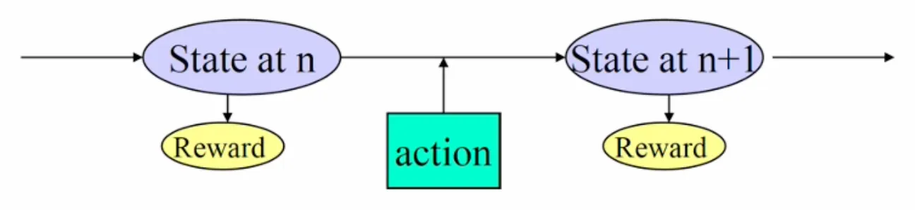
A Markov Decision Process (MDP) is a mathematical framework for modeling decision-making in situations where outcomes are partly random and partly under the control of a decision-maker. It provides a formalism for sequential decision-making problems, where an agent interacts with an environment over a series of time steps.
Definitions
- : state of the system at time
- : action taken at time
- : Markov decision process
- : reward received when transitioning from state to state
- State transition probability when action is taken at state :
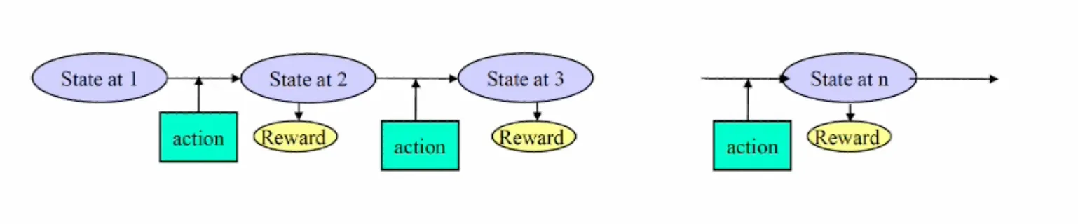
Finite State model
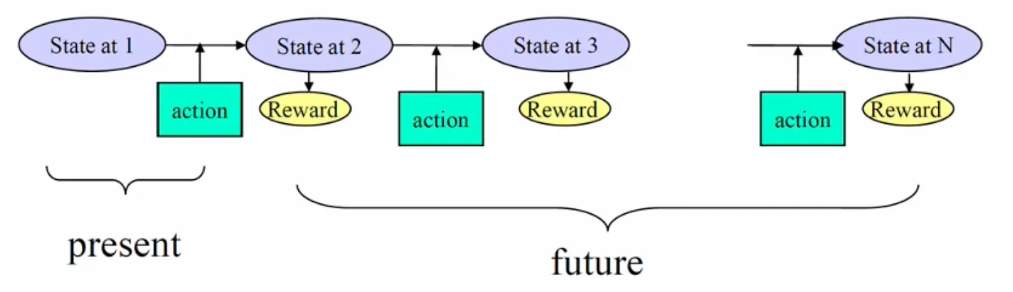
What is the optimal decision (action) at each state to maximize the expected total reward over a given time horizon?
- : optimal expected total reward when starting in state at time
- According to the principle of optimality, the optimal expected total reward can be expressed recursively as:
- Solve in order of
Example
Given three possible ad states: 0 (good), 1 (average), and 2 (bad). The advertiser can choose between two actions: a = 0 (high bid) and a = 1 (low bid). The state transition probabilities and rewards for each action are as follows:
import numpy as np
# transition probability matrices
P0 = np.array([[0.3, 0.5, 0.2], [0, 0.6, 0.4], [0, 0, 1]])P1 = np.array([[0.4, 0.5, 0.1], [0.2, 0.6, 0.2], [0.1, 0.4, 0.5]])
# reward matricesR0 = np.array([[7, 5, 2], [6, 4, 1], [3, 1, -1]])R1 = np.array([[6, 4, -1], [5, 3, -2], [4, 3, -3]])
num_states = 3 # number of statesnum_stages = 3 # number of stages (time horizon)
# initialize value functionf = {n: np.zeros(num_states) for n in range(num_stages+3)}
for n in range(num_stages, 0, -1): # backward induction for i in range(num_states): action_0 = sum(P0[i, j] * (R0[i, j] + f[n+1][j]) for j in range(num_states)) action_1 = sum(P1[i, j] * (R1[i, j] + f[n+1][j]) for j in range(num_states)) f[n][i] = max(action_0, action_1)
policy = {}for n in range(1, num_stages+1): policy[n] = [] for i in range(num_states): action_0 = sum(P0[i, j] * (R0[i, j] + f[n+1][j]) for j in range(num_states)) action_1 = sum(P1[i, j] * (R1[i, j] + f[n+1][j]) for j in range(num_states)) if action_0 >= action_1: policy[n].append(0) # choose action 0 else: policy[n].append(1) # choose action 1
print("Optimal Value Function:")for n in range(1, num_stages+1): print(f"Stage {n}: {['Action 0' if a == 0 else 'Action 1' for a in policy[n]]}")Output
Optimal Value Function:Stage 1: ['Action 0', 'Action 1', 'Action 1']Stage 2: ['Action 0', 'Action 1', 'Action 1']Stage 3: ['Action 0', 'Action 0', 'Action 1']Infinite Stage
- In a finite stage model, the optimal current action may depend on the number of remaining periods.
- However, this type of optimal policy may not be possible in an infinite stage model.
- So, the optimal policy should be only dependent on states, independently of time points, which is called a stationary policy.
- The following methods are available for obtaining stationary policy:
- Enumeration: Enumerate all possible policies and evaluate their performance.
- Policy Iteration: Start with an arbitrary policy and iteratively improve it.
- Linear Programming: Formulate the problem as a linear program and solve it.